Time Series Analysis For Business Forecasting
Time is the only moving thing in the world that never stops. When it comes to time series forecasting, the human mind tends to be more curious as we know that things change with time. Hence we are interested in making predictions ahead of time. Wherever time is an influencing factor, there is a potentially valuable thing that can be predicted. So here we are going to discuss Time Series Forecasting. Different types of forecasting we can make the machine do in real life. The name, ‘time-series’ itself suggests that data related to it varies with time. The primary motive in time series problems is forecasting. Time Series Analysis For Business Forecasting helps to forecast/predict the future values of a critical field that has a potential business value in the industry, predict the health condition of a person, predict results of a sport or performance parameters of a player based on previous performances and previous data.Time Series Forecasting Methods
Univariate Time Series Forecasting
A univariate time series forecasting problem will have only two variables. One is date-time, and the other is the field that we are forecasting. For example, if we want to predict a particular weather field, like the average temperature tomorrow, we’ll consider the temperatures of all the previous dates and use them in the model to predict for tomorrow.Multivariate Time Series Forecasting
In the multivariate case, the target would be the same, if we consider the above example as univariate, our goal is the same to predict the average temperature for tomorrow, the difference is we use all other scenarios too in the model, which affect the temperature like there is a chance for rainfall, if yes, what will be the duration of the rain? What’s the wind speed at various times? Humidity, atmospheric pressure, precipitation, solar radiation, and many more. All these factors are intuitively relevant to temperature. The primary point of consideration in comparison of univariate and multivariate is that multivariate is more suited for practical scenarios.Time Series Forecasting Models
ARIMA Model
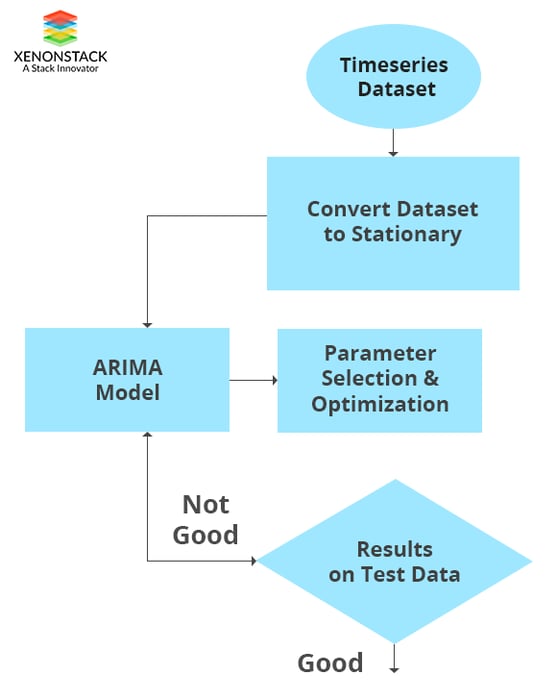
ARIMA means Autoregressive Integrated Moving Average. The AR part of ARIMA indicates that the evolving variable of interest is regressed on its own lagged (i.e., prior) values. The MA part suggests that the regression error is a linear combination of error terms whose values occurred contemporaneously and at various times in the past. The I (for "integrated") indicates that the data values have been replaced with the difference between their values and the previous values (and this differencing process may have been performed more than once). The purpose of each of these features is to make the model fit the data, and its advantage is that it depends on the accuracy over a broad domain of time series despite being more complicated.ARCH/GARCH Model
Most importantly, volatility models for time series are Autoregressive Conditional Heteroscedasticity (ARCH) and extended to its generalized version of the GARCH model. These models are very well trained in capturing dynamics of volatility from time series. Univariate GARCH models have achieved fame in volatility models, but Multivariate GARCH is still very challenging to implement in the time series.Vector Autoregression (VAR) Model
VAR is an abbreviation for Vector Autoregression. The VAR model captures the interdependencies among various time series in the data. This model is the generalization of the Univariate Autoregression Model.LSTM Model
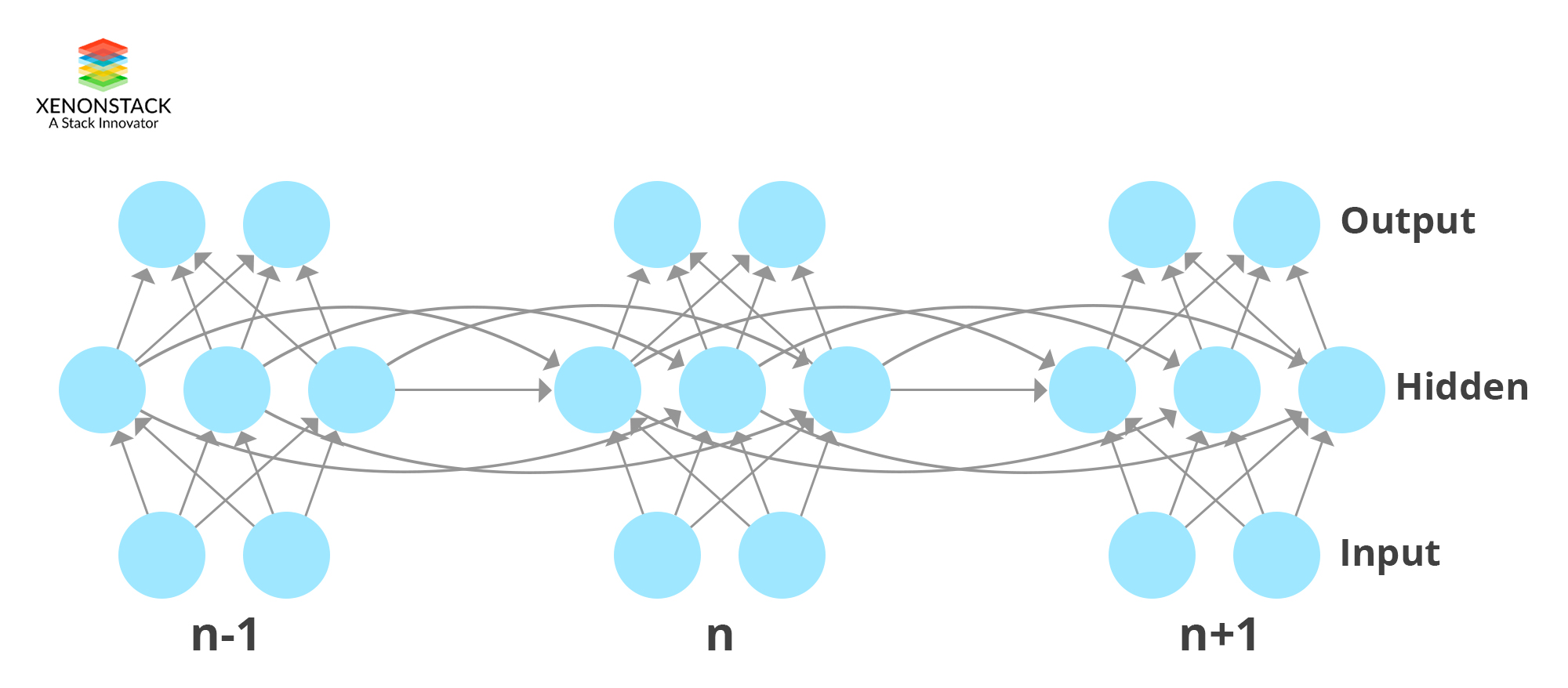
LSTM stands for long short-term memory, and it is a Deep Learning Model. LSTM is a type of Recurrent Neural Network(RNN), and RNNs are designed to capture sequence dependence. LSTM is capable of handling large architectures during training.
You May also Love to Read Automatic Log Analysis using Deep Learning and AI for Microservices
Elman and Jordan Neural Network
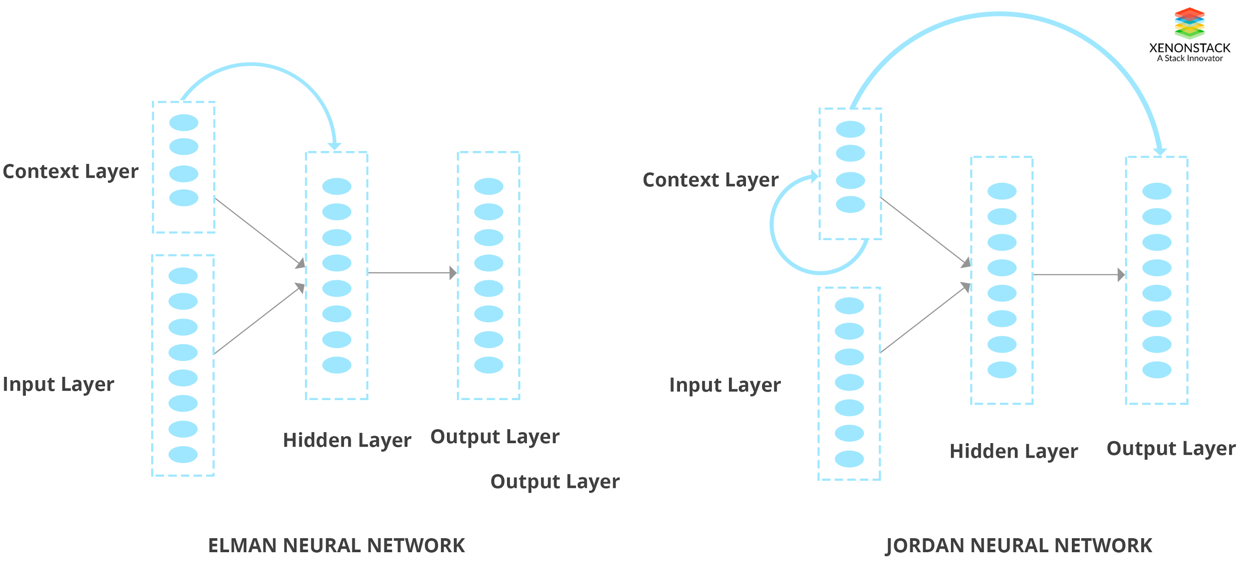
Elman and Jordan's neural networks are two types of architectures of Recurrent Neural Networks (RNN). These networks combine the past values of the context unit with the current input to obtain the final output. The Jordan context unit acts as a low pass filter, which creates an output that is the standard value of some of its most current history outputs. In these networks, the weighting over time is inflexible since we can only control the time decay. Also, a small change in time is reflected as a significant change in the weighting. Elman network is context units added to three layers network. In this, the hidden layer is connected to these context units fixed with the weight of one. At each step of this, when the input is fed forward, the learning rule is applied. Jordan network is the same as Elman, but context units are fed from the output layer instead of the hidden layer.
Approaches To Time Series Analysis
Let us assume data with a mixture of both continuous and categorical columns, and we have to forecast a column named ‘value, ’ and this column is continuous. Let the number of columns in the dataset be 100 named as ‘col1’,’col2’,’col3’... ’col100’. Along with this let, there is a categorical column ‘cat’ with ten different categories. Let us assume that each unique item in this ‘cat’ column represents a unique sensor. So, there are ten sensors, and we are getting data from all ten sensors in real-time, which produces data for the other 100 columns. This is now a multivariate time series problem, and we have to forecast values for the ‘value’ column. The later sections describe various approaches to go on with a dataset of this kind.Questions to be asked about Data
- How fast are we getting the data? (once in a second, minute, hour).
- Are all the sensors giving data at the same time or are different sensors giving data at different times?
- Are the values of the sensors related or independent?
- To predict one's future value, should we consider all the past data or the latest subset enough? If we are considering just a subset, how much data is good enough for future predictions?
Approach 1
Univariate Model
In this approach, we consider the time and the field which we are forecasting. Before modeling, we have to do some data cleaning and transformation. Data cleaning includes missing value imputation, outlier detection, and replacement. Data transformation is required to convert non-stationary time series to stationary time series. A stationary time series is one which complies with certain statistical measures like mean, variance, and autocorrelation. The data shouldn’t be heteroscedastic. That means at different intervals of time, these statistical measures are expected to be constant. In general, the data won’t be this way, so data transformation techniques like differencing, log transformation, etc. can be used to get the time series stationary.How to determine if Time Series is Stationary?
The two things that we can visualize are Trend and Seasonality. The same value of the mean with varying time denotes a constant trend. Variations in specific time intervals denote seasonality. To capture the trend, we can create a rolling mean for the data and see how the rolling mean in varying with time. Rolling mean can be explained as taking the mean of the previous few values and taking the average to define the next rolling mean value. To get the rolling mean value at n, we take an average of time series values of n-1 to n-10. If the rolling mean stays constant, we can say that that trend is in consensus with stationarity. To eliminate trends, we can use a log transformation. Along with rolling mean, we could also take care of rolling standard deviation. To test the stationarity of a time series, we can use the Dickey-Fuller test. Another method that can be used to eliminate both trend and seasonality is Differencing. Differencing is simply taking the difference between the present value and the previous value. This is also called first-order differencing.
You May also Love to Read Log Analytics, Log Mining and Anomaly Detection with AI, Deep Learning
Time Series Forecasting
We could use ARIMA (Autoregressive integrated moving average) for forecasting. ARIMA has two parameters ‘p’ and ‘q.' The value ‘p’ for AR and ‘q’ for MA. ‘p’ is the lags considered for the dependent variable. If ‘p’ is 10, for predicting the value at time t, we use values of t-1 to t-10 as predictors. ‘q’ is similar to ‘p.' The only difference is instead of taking the values, we take the forecast errors in prediction. We can model AR and MA separately and combine them for forecasting. After the modeling is finished, the values are back-transformed or inversely transformed to get the predictions to the original scale. In our case, the data has 100 columns with a mixture of both continuous and categorical values, and the data is collected from multiple sensors at different times. So, using the Univariate analysis to forecast the value column may not be sufficient for reasonable predictions. However, if there are no good relations between dependent and all independent variables and each sensor data is independent of others, we could still consider using univariate analysis for each sensor separately.Approach 2
Multivariate Model using VAR
In a multivariate model, we consider multiple columns to have the interdependencies intact and predict the values of the required field. VAR (Vector Autoregression) is a statistical technique which is a stochastic process which helps is considering all the interdependencies among various time series fields in the data. VAR is the generalization of the univariate AR model. Each variable in the model has its own lagged values to explain the predictions, and along with this it also considers other model variables too. VAR comes with parameters Akaike Information Criterion and Bayesian Information Criterion ‘AIC,' ’BIC.' These parameters are used to tune the model to select the best for the data.Approach 3
Multivariate Time Series Forecasting Using Deep Learning Keras
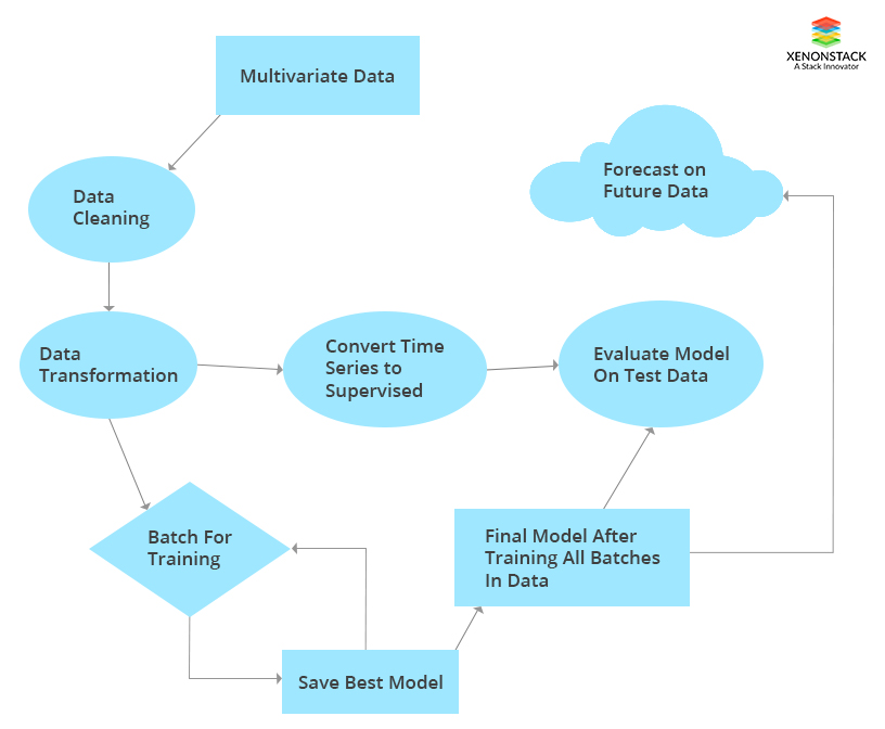
We could use Deep Learning techniques for time series forecasting. In years, sequential models with LSTM (Long short term memory) can be used for time series forecasting. LSTMs are one of the recurrent neural networks (RNN). Recurrent neural networks consider the dependency of the sequence in which the data is being inputted. Besides this, LSTM has the capability of handling huge data. The deep learning models also have the support of learning in batches, saving and reusing them with the new data to continue the training process. To implement the LSTM for multivariate data, we should convert the time series problem to a supervised learning problem. In this approach, to predict one's future value of a given field, we require values of the other variables too. So, in a way we have to predict all the other values too before predicting the required field. We could employ many methods for this, and among them one of the methods is, to predict one's future value in an independent variable, we could find the average of previous few values. To predict 10 future values, we could loop over the process for ten times. Another technique is to implement the univariate time series for each variable, and once we have future data for all the independent variables, we could use LSTM for training. Besides this, we can use the approach to train huge dataset in batches. We can work out with the number of hidden layers, other parameters during the model fitting to get the best model.
Model-Based Approach For Sensor Data Monitoring
Since the data is huge, we could use Deep Learning architecture as in the third approach to the learning process. Besides this, we could use label encoding and one hot encoding technique to transform the categorical columns and fit them into the model. Another option is, if each sensor is independent of others, we can model each sensor's data separately. In the process, we can dynamically apply cleaning and data transformation techniques and do inverse transformation after prediction to get the predictions on the correct scale.Multivariate Model With VAR and Deep Learning
In the VAR model, we need not consider converting the data to the supervised learning problem. We can directly use the VAR model to predict future values of the required column. In the Deep Learning approach, we require the values of the independent variables. VAR model cannot handle huge data at a time, whereas deep learning architecture is better at performance.Concluding Time series forecasting
Time series forecasting is similar to any other prediction with an extra complexity called time. Since time is involved, the value at two different times of output may be different even if all the input values are the same. That is a major difference. For this, the training of the model cannot be with a random shuffle, it has to be in sequence. With advances in computational power, technology, and modeling like Deep Learning, time-series data can be handled with more data with better speed and accuracy. Numerous approaches give the flexibility to choose the best according to the data.How Can XenonStack Help You?
Advanced Analytics Solutions
XenonStack Data Science As-A-Service provides Cognitive & Prescriptive Intelligence to Automate Analytical Model Building using Machine Learning, Deep Learning, and Artificial Intelligence for Image Classification, Speech Recognition, Fraud Detection, Anomaly Detection, Risk Prediction, Energy Optimization, and Natural Language Recognition.Machine Learning and Deep Learning on Kubernetes
XenonStack IT Infrastructure & DevOps expertise helps you to Build & Deploy the model in production based on Performance Requirements and Optimization of the Model. XenonStack Machine Learning Solutions, Deep Learning Solutions, and Docker Solutions help you to Deploy Machine learning and Deep Learning Models (Python & R Models) on Docker and Kubernetes.Decision Science Solutions
XenonStack Data Visualization & Artificial Intelligence Services enables you to develop an Interactive Dashboard, Data Product in the form of Chat Bots, Digital Agents and Decision Science framework, and recommendation systems with progressive web Applications Using Angular.JS, React.JS, and Reactive Programming – Scala, GoLang.
- Learn more about Predictive Analytics Tools and Techniques
- Get an Insight into Predictive Analytics Solution for Healthcare and Insurance
.webp?width=1921&height=622&name=usecase-banner%20(1).webp)


